File: Time_Series
Analysis.xls
Features
Time series data are
analyzed for user-defined sites, variables, & time
intervals.
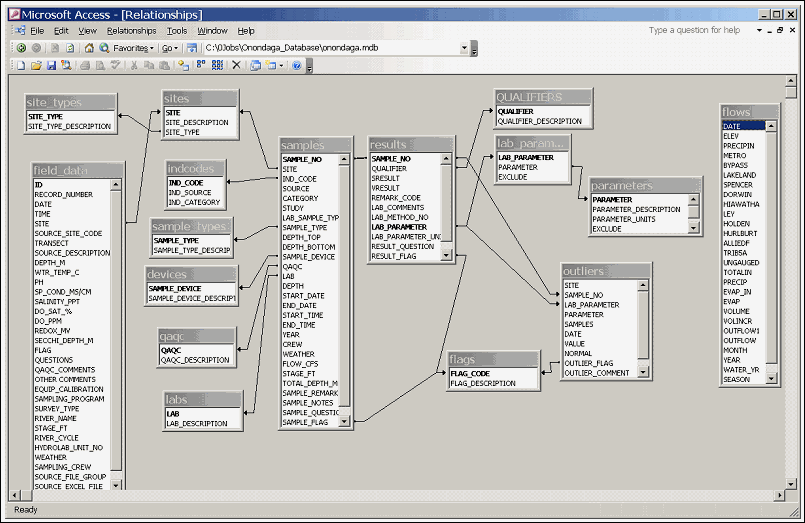
Concentration and flow data are retrieved from the access database (master_filtered query).
Statistical outliers are identified for potential flagging in the database.
Trend analyses are conducted using the Seasonal Kendall test.
Results are summarized in various charts and tables that can be archived and later reviewed .
See general instructions for installation and
operation.
Execution for a Single Site
& Variable
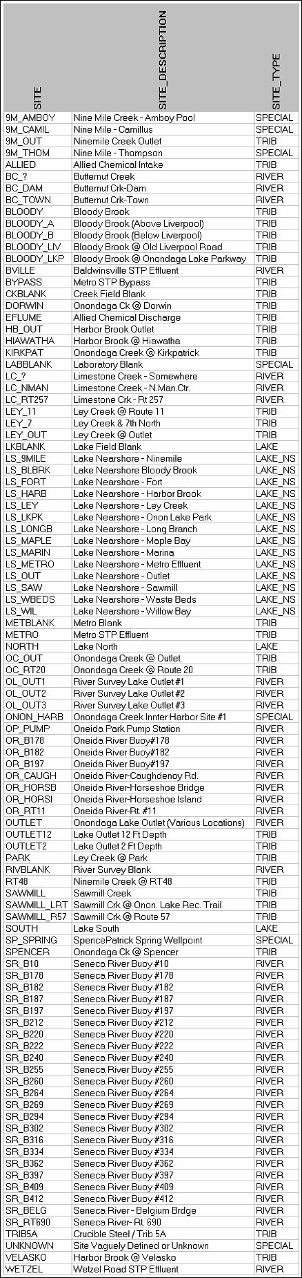
Review the Site_Index sheet. The listed site codes must be
registered in the sites table of the access
database.
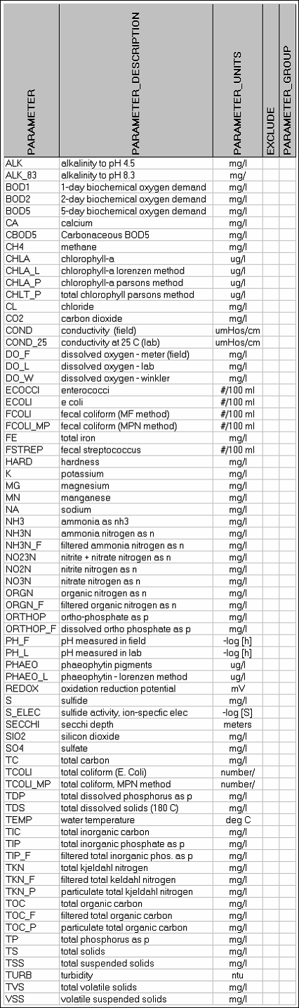
Review Variable_Index sheet. The listed parameter codes must be registered in the parameters table of the database, which is, in turn, linked to lab_parameter codes stored in the results file.
Review input parameters in the red cells below the menu & edit if desired.
Set date range for the analysis (typically >= 10 years in length).
Set date range for tabulating outliers. When updating the database, this would normally be the most recent year.
Select a site and water quality parameter from the windows.
Select a transformation option: default (specified in parameter index), linear, or log.
Select Run For: "Selected Site & Variable"
Click the "Run" button.
The outlier and trend analyses are performed simultaneously.
Results are summarized in the table and graphs to the right of the menu page.
Review other output pages & graphs selected from the
output sheets window.
Execution for Multiple Sites & Variables ("Batch Run")
The analysis can be
performed for multiple sites and or variables in
sequence.
Select sites by entering '1' in the 'Batch' column of the site_index sheet.
Select variables by entering '1' in the 'Batch' column of the variable_index sheet.
Batch runs automatically use the transformations.
Check or uncheck option to publish batch results. For each variable & site combination, a snapshot of the graphs on the right side of the menu screen is saved in gif format. The files are stored in a subdirectory of the database specified below the menu screen.
Select the "Run for" option:
(2) Selected Variable & Each Site
(3) Selected Site & Each Variable
(4) All Sites & Variables
Click the "Run" Button.
The procedure runs for each site and variable combination.
Output can be viewed from the sheet menu in the "Batch Results" section.
Click 'Save Batch Results' to store output tables in a separate workbook for archiving.
Click the 'Update Chart Catalogue' button to make a series of
batch runs that will update all charts in the library accessed from the
view_output.xls. Output includes chart
arrays grouped by site and variable. Loops through each combination of
site & variable twice.
Transformations
Log transformation of the concentration data is often
appropriate before performing parametric statistical procedures that assume a
normal distribution, such as the outlier detection procedure. Trend
analysis results are insensitive to the transformation because a non-parametric
procedure is used.
Default transformation options are specified for each variable on the variable index sheet. For as single site/variable analysis, the defaults can be over-ridden by selecting a linear or log transform option on the menu screen. Batch runs for multiple sites and variable use the default transformations.
If a log transformation is elected, '0' values in the data set are set equal to the lowest positive value.
The variable index sheet also allows specification of a
minimum value for each parameter. This can help to eliminate negative
skewness that occurs when log transformed datasets contain a few extremely low
values
Trend
Analysis
Trend analysis is
performed using a test developed by Hirsch & Slack
(1984). Fortran code was developed for another
application (Walker, 1991), used in analyzing the
1968-1991 Onondaga Lake database and subsequently
adapted for OCDWEP use in preparing lake monitoring reports (Walker, 1995). The
software has been converted to VBA (Excel macro language) and tested against the
original software.
Data are grouped by "seasons" within each year Season length (days<=52) is specified in the input parameters section of the menu sheet. Generally, the length of each "season" should be equal to or greater than the typical sampling interval. For example, with a biweekly sampling frequency, the number of seasons would be <= 26. A monthly analysis (seasons = 12) is typical.
Results of hypothesis tests ("p levels") are computed using two versions of the test. One version (Hirsch et al, 1982 ) ignores serial correlation. The other version (Hirsch & Slack, 1984) accounts for it. The latter, more conservative test has been routinely used in lake monitoring reports.
To classify the results into two categories (significant, not significant), the user must select which test to use (default = second test) and the significance level (default = 0.1). These choices are made in cells below the menu screen. They influence only the final cross-tabulation of 'significant trends' accessed via the sheet index on the menu screen.
Other options are specified in the input parameters section of the menu screen. Three options are available for summarizing data within each season and year (mean, median (recommended), or middle value, in time sequence).
Via the checkbox on the menu screen, the user has the option to exclude outliers from the trend analysis. While this may shrink the scales of the output time series to elucidate trends, it will generally not affect the results of Seasonal Kendall test because of its robust features.
The final tabulation of significant trends should not be accepted without first reviewing the individual time series plots. The trend analysis may produce erroneous results in datasets with significant data gaps, high frequencies of values at or below detection, or a shift in the detection limit. This situation occurs for BOD-5 and NH3-N at some sites.
Outlier Screening
The primary purpose
for the outlier screening is to provide additional quality control for data
entry and transfer to the database. Errors may be identified and
corrected in the process of verifying a results rejected by the outlier
routine. As described below, remaining outliers can be flagged in the
database at two levels (provisional or fatal). Flags, in turn, may limit
subsequent data retrieval, depending upon the employed.
In screening of the 1968-2002 data, ?% of the results were rejected. Of these, ?% were accepted (see discussion below regarding snowmelt samples) and ?% were assigned provisional flags. None were assigned fatal flags. Preliminary runs identified many results that reflect data entry or transmittal errors that were subsequently corrected in the database.
The outlier screening algorithm is adapted from Gilbert(1987) .The data are fit to a normal or lognormal distribution using a procedure that is robust to outliers. The assumed distribution type is specified by the user in the variable index. If a log transformation is selected, all plots are generated with log scales.
The sample time series is filtered to remove seasonal variations and long-term trend before testing for outliers. Filtering subtracts the seasonal median (over all years) and uses the slope of the trend line to detrend the data. The distribution is fit based to the 16th, 50th, and 80th percentile values of the transformed (if elected) and filtered data.
A sample is rejected if the tail probability is less than a / N, where a = user-defined significance level, and N = number of observations.
Outlier time series plots show filtered values and rejection limits. Limits depend on N, but are generally 4-5 times the standard deviation for a = 0.01
Outliers are listed for single & batch runs on separate
sheets.
Updating the Outliers Table in the Access
Database
Set the date range for listing outliers in most
recent year.
If desired, check the 'Plot Series with Outliers Only' box. This will restrict the 'Outlier Time Series' page to include only plots with detected outliers for the most recent year.
Run for all sites & all variables.
Review the batch outlier listing & corresponding graphs (outlier time series and histograms in the batch output section of the menu)
The outlier crosstab identifies samples with outliers for one or mores.
Review source records in database to check for data entry errors etc., make any corrections, and repeat the analysis.
Copy outlier listing sheet to the end of the outliers table in the 'Outliers.xls' file. This table is linked to access database and contains results for all years.
Classify the new records in three categories using the
"Outlier_Flag" column:
0 or blank accept sample*
1 provisional flag (result a-typical but still retrieved in queries)
2
fatal flag (rejected result, not
retrieved in queries)
The procedure will occasionally reject samples that are actually representative if the frequency distribution deviates significantly from a normal distribution or if the time series is strongly event-driven. For example, tributary samples with elevated chloride and sodium were frequently identified in screening the historical data. These tended to occur simultaneously and during the winter months. The pattern indicates that these samples reflect snowmelt events. The samples remain in the outlier table, but the flag field is blank, so the data are routinely retrieved.