BATHTUB Overview
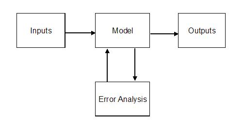
A flow diagram for BATHTUB calculations is shown in Figure 1:
|
|
Using a first-order error analysis procedure (Walker 1982), the model core is executed repeatedly in order to estimate output sensitivity to each input variable and submodel and to develop variance estimates and confidence limits for each output variable. The following section describes calculations performed in the model core.
 |
Control pathways for predicting nutrient levels and eutrophication response in a given model segment are illustrated in Figure 2. Predictions are based upon empirical models which have been calibrated and tested for reservoir applications (Walker 1985). Model features are documented as follows:
Table 1 Symbol Definitions
Table 2: Model Equations and Options
Table 3: Diagnostic Output Variables
Table 4: Error Statistics
Several options are provided for modeling nutrient sedimentation, chlorophyll a, and transparency (Table 2). In each case, Models 1 and 2 are the most general formulations, based upon model testing results. Alternative models are included to permit sensitivity analyses and application of the program under various data constraints. Table 2 also specifies equations for predicting supplementary response variables (organic nitrogen, particulate phosphorus, principal components, oxygen depletion rates, trophic state indices, algal nuisance frequencies), as calibrated to CE reservoir datasets. Diagnostic output variables that reflect various aspects of reservoir trophic state are described in Table 3. Error statistics for applications of the model network to predict spatially averaged conditions are summarized in Table 4.
Research reports (Walker, 1981, 1982, 1985 ) describe the datasets, underlying theory, development, and testing of the network equations. These should be reviewed prior to using the program. The following sections summarize underlying concepts.
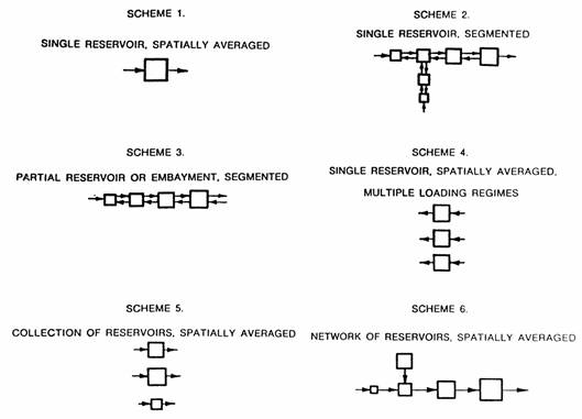
Through appropriate configuration of model segments, BATHTUB can be applied to a wide range of reservoir configurations and management problems. Figure 3 depicts segmentation schemes in six general categories:
Segments can be modeled independently or linked in a network. Each segment is defined in terms of its morphometry (area, mean depth, length, mixed layer depth, hypolimnetic depth) and observed water quality (optional). Morphometric features refer to average conditions during the period being simulated. Segment linkage is defined by assigning each segment an ID number (from 1 to 50) and specifying the segment that is immediately downstream. Multiple external sources and/or withdrawals can be specified for each segment. With certain limitations, combinations of the above schemes are also possible. Characteristics and applications of each segmentation scheme are discussed below.
Scheme 1 (Figure 3) is the simplest configuration. It is applicable to reservoirs in which spatial variations in nutrient concentrations and related trophic state indicators are relatively unimportant. It can also be applied to predict area-weighted mean conditions in reservoirs with significant spatial variations. This is the simplest type of application, primarily because transport characteristics within the reservoir (particularly, longitudinal dispersion) are not considered. The development of submodels for nutrient sedimentation and eutrophication response has been based primarily upon application of this segmentation scheme to spatially averaged data from 41 CE reservoirs (Walker 1985).
Scheme 2 involves dividing the reservoir into a network of segments for predicting spatial variations in water quality. Segments represent different areas of the reservoir (e.g., upper pool, middle pool, near dam). Longitudinal nutrient profiles are predicted based upon simulations of advective transport, diffusive transport, and nutrient sedimentation. Reversed arrows in Figure 4.3 reflect simulation of longitudinal dispersion. Branches in the segmentation scheme reflect major tributary arms or embayments. Multiple and higher order branches are also permitted. Segment boundaries can be defined based upon consideration of the following:
Reservoir morphometry
Locations of major inflows and nutrient sources
Observed spatial variations in water quality
Locations of critical reservoir use areas
Numerical dispersion potential (calculated by the program)
If pool monitoring data are available, spatial displays generated by PROFILE (Walker, 1999 ) can be useful for identifying appropriate model segmentation. A degree of subjective judgment is normally involved in specifying segment boundaries, and sensitivity to alternative segmentation schemes should be investigated. Sensitivity to assumed segmentation should be low if longitudinal transport characteristics are adequately represented. Experience with the program indicates that segment lengths on the order of 5 to 20 km are generally appropriate, but this range may vary with the size and shape of the reservoir. Segmentation should be done conservatively (i.e., use the minimum number required for each application).
Scheme 3 illustrates use of BATHTUB for modeling partial reservoirs or embayments. This is similar to Scheme 2, except the entire reservoir is not being simulated and the downstream water quality boundary condition is fixed. Diffusive exchange with the downstream water body is represented by the bidirectional arrows attached to the last (most downstream) segment. An independent estimate of diffusive exchange with the downstream water body is required for this type of application.
Scheme 4 involves modeling multiple loading scenarios for a single reservoir in a spatially-averaged mode. Each �segment� represents the same reservoir, but under a different �condition,� as defined by external nutrient loading, reservoir morphometry, or other input variables. This scheme is useful primarily in a predictive mode for evaluation and rapid comparison of alternative management plans or loading scenarios. For example, Segment 1 might reflect existing conditions; Segment 2 might reflect projected future loadings as a result of land development; and Segment 3 might reflect projected future loadings with specific control options. By defining segments to reflect a wide range of loading conditions, loadings consistent with specific water quality objectives (expressed in terms of mean phosphorus concentration, chlorophyll a, and/or transparency) can be identified. One limitation of Scheme 4 is that certain input variables, namely precipitation, evaporation, and change in storage, are assumed to be constant for each segment. If year-to-year variations in these factors are significant, a separate input file should be constructed for each year.
Scheme 5 involves modeling a collection of reservoirs in a spatially averaged mode. Each segment represents a different reservoir. This is useful for regional assessments of reservoir conditions (i.e., rankings) and evaluations of model performance. Using this scheme, a single file can be set up to include input conditions (water and nutrient loadings, morphometry, etc.) and observed water quality conditions for each reservoir in a given region (e.g., state, ecoregion). As for Scheme 4, a separate input file must be constructed for each reservoir if there are significant differences in precipitation, evaporation, or change in storage across reservoirs.
Scheme 6 represents a network of reservoirs in which flow and nutrients can be routed from one impoundment to another. Each reservoir is modeled in a spatially averaged mode. For example, this scheme could be used to represent a network of tributary and main stem impoundments. This type of application is feasible in theory but has been less extensively tested than those described above. One limitation is that nutrient losses in streams linking the reservoirs are not directly represented. Such losses may be important in some systems, depending upon such factors as stream segment length and time of travel. In practice, losses in transport could be approximately handled by defining �stream segments,� provided that field data are available for calibration of sedimentation coefficients (particularly in the case of nitrogen). Networking of reservoirs is most reliable for mass balances formulated on a seasonal basis and for reservoirs that are unstratified or have surface outlets.
As illustrated in Figure 3, a high degree of flexibility is available for specifying model segments. Combinations of schemes are also possible within a given input file. While each segment is modeled as vertically mixed, BATHTUB is applicable to stratified systems because the formulations have been empirically calibrated to data from a wide variety of reservoir types, including well-mixed and vertically stratified systems. Effects of vertical variations are incorporated in the model parameter estimates and error terms.
As indicated in Table 2, nutrient sedimentation coefficients may depend upon morphometric and hydrologic characteristics. To provide consistency with the data sets used in model calibration, segments must be aggregated for the purpose of computing effective sedimentation rate coefficients (A1 and B1 in Table 2). A �Segment Group Number� is defined for this purpose. Rate-coefficient computations are based upon the following variables summarized by segment group:
Surface overflow rate
Flushing rate (1 / hydraulic residence time)
Total external nutrient load.
Tributary total nutrient load
Tributary ortho-P or inorganic nitrogen load.
Flushing rate is also used in chlorophyll a Models 1 and 2 . Area-weighted mean chlorophyll a values are computed for each segment group and used in the computation of hypolimnetic oxygen depletion rates (see Table 2).
Group numbers are integers ranging from 1 up to the total number of segments defined for the current case. Generally, if a case involves simulation of a single reservoir with multiple segments, all segments should be assigned the same group number (1). If the segments represent reservoir regions (tributary arms) with distinctly different morphometric, hydrologic, and water quality characteristics, different group numbers can be assigned to each region. If the case involves simulation of multiple reservoirs (Schemes 5 or 6 in Figure 3), different group numbers are assigned to each reservoir.
Multiple of external inflows (�Tributaries�) can be specified for any model segment. Tributaries are identified by name and a sequence number between 1 and 99. Each tributary is assigned to a specific segment number and classified using the following Type Codes :
1 - Monitored Inflow
2 - Nonpoint
Inflow
3 - Point-Source
Inflow
4 - Outflow or
Withdrawal
5 - Diffusive
Source
Type 1 describes tributaries with inflow volumes and nutrient concentrations that are directly monitored or otherwise estimated. Type 2 describes watershed areas that are not monitored; inflow volumes and concentrations are estimated from user-defined landuse categories and export coefficients. In order to invoke this tributary type, the user must supply independent estimates of export coefficients (runoff (m/year) and typical runoff concentrations for each land use) developed from regional data. Type 3 describes point sources (e.g., wastewater treatment plant effluents) that discharge directly to the reservoir. Type 4 describes measured outflows or withdrawals; these are optional, since the model predicts outflow from the last segment based upon water-balance calculations. Specification of outflow streams is useful for checking water-balance calculations (by comparing observed and predicted outflow volumes). Type 5 defines diffusive exchange with downstream water bodies in simulating embayments (e.g., Scheme 3 in Figure 3).
In normal segmentation schemes, outflow from each segment discharges to the next downstream segment or out of the system. An option for specifying additional advective and/or diffusive transport between any pair of segments is also provided. A maximum of 10 �Transport Channels� can be defined for this purpose. Independent measurements or estimates of advective and/or diffusive flow are required to invoke this option. Definition of transport channels is not required for simulating typical one-dimensional branched networks in which each segment discharges only to one downstream segment.
The mass-balance concept is fundamental to reservoir eutrophication modeling. BATHTUB formulates water and nutrient balances by establishing a control volume around each segment and evaluating the following terms:
Inflows = Outflows + Increase-in-Storage + Net Loss
Inflow Terms = External Inflow + Advective + Diffusive + Precipitation
Outflow Components = Discharge from Reservoir + Advective + Diffusive + Evaporation
The external, atmospheric, discharge, evaporation, and increase-in-storage terms are calculated directly from information provided by the user in the input file. The remaining are discussed below.
Advective terms reflect net discharge from one segment into another and are derived from water-balance calculations. Diffusive transport terms are applicable only to problems involving simulation of spatial variations within reservoirs. They reflect eddy diffusion (as driven by random currents and wind mixing) and are represented by bulk exchange flows between adjacent segment pairs. Chapra and Reckhow (1983) present examples of lake/embayment models that consider diffusive transport.
Five methods are available for estimating diffusive transport rates (Table 2). Each involves calculation of bulk exchange flows which occur in both directions at each segment interface. Dispersion coefficients, calculated from the Fischer et al. (1979) equation (Model 1) or from a fixed longitudinal dispersion coefficient (Model 2), are adjusted to account for effects of numeric dispersion (�artificial� dispersion or mixing that is a consequence of model segmentation). Model 3 can be used for direct input of bulk exchange flows.
Despite its original development based upon data from river systems, the applicability of the Fischer et al. equation for estimating longitudinal dispersion rates in reservoirs has been demonstrated previously (Walker 1985 ). For a given segment width, mean depth, and outflow, numeric dispersion is proportional to segment length. By selecting segment lengths to keep numeric dispersion rates less than the estimated values, the effects of numeric dispersion on the calculations can be approximately controlled. Based upon Fischer�s dispersion equation, the numeric dispersion rate will be less than the calculated dispersion rate if the following condition holds:
L < 200 W2 Z-0.84
where,
L =
segment length, km
W = mean top width = surface area/length,
km
Z = mean depth,
m
The above
equation can be applied to reservoir-average conditions in order to estimate an
upper bound for the appropriate segment length. In most cases, simulated
nutrient profiles are relatively insensitive to longitudinal dispersion
rates. Fine-tuning of exchange flows can be achieved via the use of
segment-specific calibration factors.
While, in theory, the increase-in-storage term should reflect both changes in pool volume and concentration, only the volume change is considered in mass-balance calculations, and concentrations are assumed to be at steady state. The increase-in-storage term is used primarily in verifying the overall water balance. Predictions are more reliable under steady pool levels or when changes in pool volume are small in relation to total inflow and outflow.
For a water balance or conservative substance balance, the net sedimentaion term is zero. Nutrient retention models are used to estimate net removal of phosphorus or nitrogen in each segment according to the equations specified in Table 2. Based upon research results, a second-order decay model is the most generally applicable formulation for representing phosphorus and nitrogen sedimentation in reservoirs:
Ws = K2 C2
where,
Ws = nutrient
sedimentation rate, mg/m3-year
K2 = effective second-order
decay rate, m3/mg-year
C = pool nutrient concentration,
mg/m3
Other options are provided for users interested in testing alternative models. The default model error coefficients supplied with the program, however, have been estimated from the model development data set using the second-order sedimentation formulations. Accordingly, error analysis results (predicted coefficients of variation) will be invalid for other formulations (i.e., Models 3 through 7 for phosphorus or nitrogen), unless the user supplies independent estimates of model error terms.
Effective second-order sedimentation coefficients are on the order of 0.1 m3/mg-year for total phosphorus and 0.0032 m3/mg-year for total nitrogen ( P & N Model 3 in Table 2 ). With these coefficients, nutrient sedimentation models explain 83 and 84 percent of the between-reservoir variance in average phosphorus and nitrogen concentrations, respectively. Residuals from these models are systematically related to inflow nutrient partitioning (dissolved versus particulate or inorganic versus organic) and to surface overflow rate over the data set range of 4 to 1,000 m/year. Effective rate coefficients tend to be lower in systems with high ortho-P/total P (and high inorganic N/total N) loading ratios or with low overflow rates (4 to 10 m/year). Refinements to the second-order formulations (Models 1 and 2) are designed to account for these dependencies (Walker 1985).
Nutrient Sedimentation Models 1 and 2 use different schemes to account for effects of inflow nutrient partitioning. In the case of phosphorus, Model 1 performs mass balance calculations on �available P,� a weighted sum of ortho-P and non-ortho-P which places a heavier emphasis on the ortho-P (more biologically available) component. Model 2 uses total phosphorus concentrations but represents the effective sedimentation rate as inversely related to the tributary ortho-P/total P ratio, so that predicted sedimentation rates are higher in systems dominated by nonortho (particulate or organic) P loadings and lower in systems dominated by ortho-P or dissolved P loadings. The nitrogen models are structured similarly, although nitrogen balances are much less sensitive to inflow nutrient partitioning than are phosphorus balances, probably because inflow nitrogen tends to be less strongly associated with suspended sediments.
Model 1 accounts for inflow nutrient partitioning by adjusting the inflow concentrations, and Model 2 accounts for inflow nutrient partitioning by adjusting the effective sedimentation rate coefficient. While Model 2 seems physically reasonable, Model 1 has advantages in reservoirs with complex loading patterns because a fixed sedimentation coefficient can be used and effects of inflow partitioning are incorporated prior to the mass balance calculations. Because existing data sets do not permit general discrimination between these two approaches, each method should be tested for applicability to a particular case. In most situations, predictions will be relatively insensitive to the particular sedimentation model employed, especially if the ortho-P/total P loading ratio is in a moderate range (roughly 0.25 to 0.60). Additional model application experiences suggest that Method 2 may have an edge over Model 1 in systems with relatively long hydraulic residence times (roughly, exceeding 1 year), although further testing is needed. Because the coefficients are concentration- or load-dependent and because the models do not predict nutrient partitioning in reservoir outflows, Sedimentation Model 2 cannot be applied to simulations of reservoir networks (Scheme 6 in Figure 4.3).
Based upon error analysis calculations , the models discussed above provide estimates of second-order sedimentation coefficients which are generally accurate to within a factor of 2 for phosphorus and a factor of 3 for nitrogen. In many applications, especially reservoirs with low hydraulic residence times, this level of accuracy is adequate because the nutrient balances are dominated by other terms (especially, inflow and outflow). In applications to existing reservoirs, sedimentation coefficients estimated from the above models can be adjusted within certain ranges (roughly a factor of 2 for P, factor of 3 for N) to improve agreement between observed and predicted nutrient concentrations. Such �tuning� of sedimentation coefficients should be approached cautiously because differences between observed and predicted nutrient levels may be attributed to factors other than errors in the estimated sedimentation rates, particularly if external loadings and pool concentrations are not at steady state.
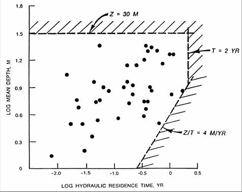 |
| Figure 4 - Mean Depth vs. Hydraulic Residence Time (Log 10 units) |
Figure 4 shows the relationship between hydraulic residence time and mean depth in the reservoir data set used for model development. Predictions of nutrient sedimentation rates are less reliable in reservoirs lying outside the data set range. This applies primarily to reservoirs with residence times exceeding 2 years, mean depths greater than 30 m, or overflow rates less than 4 m/year. Tests based upon independent data sets indicate that the sedimentation models are unbiased under these conditions but have higher error variances. In such situations, the modeling exercise should include a sensitivity analysis to model selection and, if possible, calibration of sedimentation coefficients to match observed concentration data. Deviations at the other extremes (reservoirs with lower residence times or higher overflow rates than those represented in the model development data set) are of less concern because the sedimentation term is generally an insignificant portion of the total nutrient budget in such systems (i.e., predicted pool concentrations are highly insensitive to estimated sedimentation rate).
Because the sedimentation models have been empirically calibrated, effects of �internal loading� or phosphorus recycling from bottom sediments are inherently reflected in the model parameter values and error statistics. Generally, internal recycling potential is enhanced in reservoirs with one or more of the following characteristics:
The above conditions are often found in relatively shallow prairie reservoirs; Lake Ashtabula (U.S. Army Engineer District, St. Paul) is an example included in the CE reservoir data set. In such situations, empirical sedimentation models will under-predict reservoir phosphorus concentrations. Depending upon the efficiency of the internal recycling process, steady-state phosphorus responses can be approximately simulated by reducing the effective sedimentation coefficient (e.g., roughly to 0. in the case of Ashtabula). An option for direct specification of internal loading rates is also provided for use in situations where independent measurements or estimates are available (see further discussion )
Nutrient Residence Time & Turnover Ratio
The �averaging period� is defined as the period of time over which
water and mass balance calculations are performed. The selection of an
appropriate averaging period is an important step in applying this type of model
to reservoirs. Two variables must be considered in this
process:
Mass Residence Time (yrs) = Nutrient Mass in Reservoir (kg) / External Nutrient Loading (kg/yr)
Nutrient Turnover Ratio = Length of Averaging
Period for Mass Balances (yrs) / Mass Residence Time (yrs)
Estimates of reservoir nutrient mass and external loading correspond
to the averaging period for the mass balance calculations. The turnover
ratio approximates the number of times that the nutrient mass in the reservoir
is displaced during the averaging period. Ideally, the turnover ratio should
exceed 2.0. If the ratio is too low, then pool and outflow water quality
measurements would increasingly reflect loading conditions experienced prior to
the start of the averaging period, which would be especially problematical if
there were substantial year-to-year variations in loadings.
At extremely high
turnover ratios and low nutrient residence times (<2 weeks), the
variability of loading conditions within the averaging period (as attributed to
storm events, etc.) would be increasingly reflected in the pool and outflow
water quality measurements. In such cases, pool measurement variability
may be relatively high, and the biological response (e.g., chlorophyll a
production) may not be in equilibrium with ambient nutrient levels, particularly
immediately following storm events.
|
|
|
|
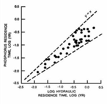
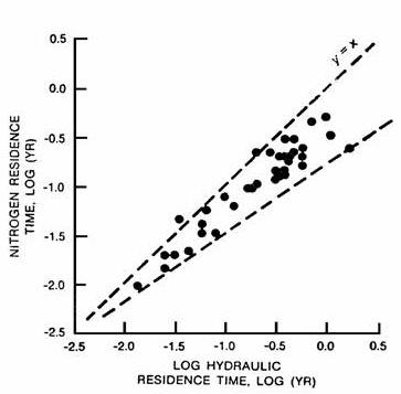
Figure 5 - Phosphorus & Nitrogen Mass Residence Time vs. Hydraulic Residence Time (Log 10 units) | |
Figure 5 shows that the hydraulic residence time is an important factor in determining phosphorus and nitrogen residence times, based upon annual mass balances from 40 CE reservoirs used in model development. For a conservative substance, the mass and hydraulic residence times would be equal at steady state. The envelopes in Figure 5 show that the spread of nutrient residence times increases with hydraulic residence time; this reflects the increasing importance of sedimentation as a component of the overall nutrient balance. At low hydraulic residence times, there is relatively little opportunity for nutrient sedimentation, and pool nutrient concentrations and residence times can be predicted relatively easily from inflow concentrations. At high hydraulic residence times, predicted pool nutrient concentrations and residence times become increasingly dependent upon the empirical formulations used to represent nutrient sedimentation. This behavior is reflected in the sensitivity curves discussed in Chapter 1.
Normally, the appropriate averaging period for water and mass balance calculations would be 1 year for reservoirs with relatively long nutrient residence times or seasonal (May-September) for reservoirs with relatively short nutrient residence times. As shown in Figure 5 , most of the reservoirs in the model development data set had phosphorus residence times less than 0.2 year, which corresponds roughly to a nutrient turnover ratio of 2 for a 5-month seasonal averaging period. Thus, assuming that the reservoirs used in model development are representative, seasonal balances would be appropriate for most CE reservoir studies. BATHTUB calculates mass residence times and turnover ratios using observed or predicted pool concentration data. Results can be used to select an appropriate averaging period for each application.
The water balances are expressed as a system of simultaneous linear equations that are solved via matrix inversion to estimate the advective outflow from each model segment. The mass balances are expressed as a system of simultaneous nonlinear equations which are solved iteratively via Newton�s Method (Burden, Faires, and Reynolds 1981). Mass-balance solutions can be obtained for up to three constituents (total phosphorus, total nitrogen, and a user-defined conservative substance). Total phosphorus and total nitrogen concentrations are subsequently input to the model network (Figure 2) to estimate eutrophication responses in each segment. Conservative substances (e.g., chloride, conductivity) can be modeled to verify water budgets and calibrate longitudinal dispersion rates.
Eutrophication Response Models
Eutrophication response models relate observed or predicted pool nutrient levels to measures of algal density and related water quality conditions. Table 3 lists diagnostic variables included in BATHTUB output, along withguidelines for their interpretation. Corresponding equations are listed in Table 2 . They can be categorized as follows:
Statistical summaries derived from the CE model development data set and listed in Table 3 provide one frame of reference. Low and high ranges given for specific variables provide approximate bases for assessing controlling processes and factors, including growth limitation by light, nitrogen, and phosphorus.
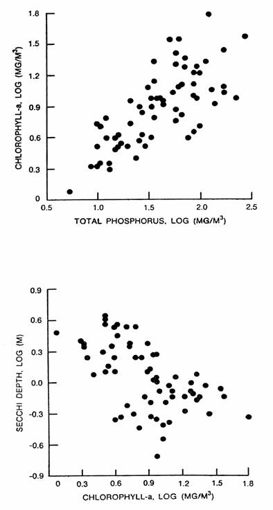
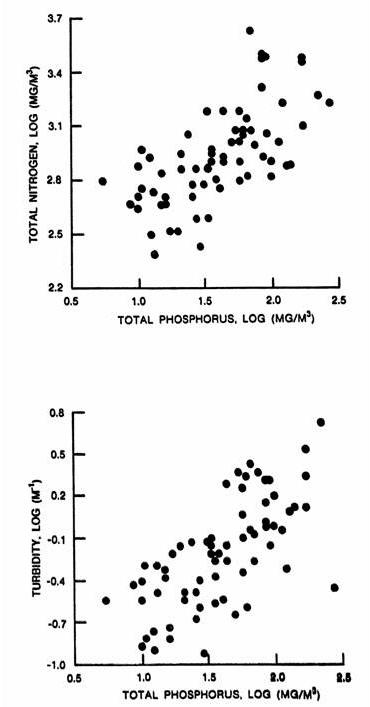
The ranges of conditions under which the empirical models have been developed should be considered in each application. Figure 6 depicts relationships among three key variables determining eutrophication responses (total phosphorus, total nitrogen, and non-algal turbidity, chlorophyll-a, and transparency). Plotting data from a given application on each of these figures permits comparative assessment of reservoir conditions and evaluations of model applicability. If reservoir data fall outside the clusters in Figure 4, 5 or 6, potential model errors are greater than indicated by the error statistics in Table 4 .
|
|
|
|
Figure 6 - Correlations Among Total P, Chlorophyll-a, Non-Algal Turbidity, Chlorophyll-a & Secchi Depth (Log 10 units) | |
The prediction of mean chlorophyll a from observed or predicted nutrient concentrations can be based on one of the five models listed in Table 4.2. Error analyses indicate that it is generally more difficult to predict chlorophyll a from nutrient concentrations and other controlling factors than to predict nutrient concentrations from external loadings and morphometry. This partially reflects greater inherent variability of chlorophyll a. Chlorophyll a models can be described according to limiting factors:
Model
Limiting
Factors
1
P, N, light,
flushing
2
P, light, flushing
3 P,
N
4
P (linear)
5
P (exponential)
Approximate applicability constraints are given in Table 2 . �Northern lake� eutrophication models are based upon phosphorus/chlorophyll regressions (similar to Models 4 and 5). Research objectives (Walker 1985) have been to define the approximate ranges of conditions under which simple phosphorus/ chlorophyll relationships are appropriate and to develop more elaborate models (Models 1-3) which explicitly account for additional controlling factors (nitrogen, light, flushing rate).
While model refinements have been successful in reducing error variance associated with simple phosphorus/chlorophyll relationships by approximately 58 percent, a �penalty� is paid in terms of increased data requirements (e.g., non-algal turbidity, mixed-layer depths, nitrogen, and flushing rate). For existing reservoirs, these additional data requirements can be satisfied from pool monitoring and nutrient loading information. Otherwise, estimates must be based upon subjective estimates, independent hydrodynamic models, and/or regional data from similar reservoirs. Empirical models for developing independent estimates of turbidity, mixed-layer depth, and mean hypolimnetic depth are summarized in Table 4.6. These should be used only in the absence of site-specific measurements.
Since mechanistic models for predicting nonalgal turbidity levels as a function of deterministic factors (e.g., suspended-solids loadings and the sedimentation process) have not been developed, it is possible to predict chlorophyll a responses to changes in nutrient loading in light-limited reservoirs only under stable turbidity conditions. Projections of chlorophyll a concentrations should include a sensitivity analysis over a reasonable range of turbidity levels.
Estimates of non-algal turbidity in each segment (minimum = 0.08 m-1) are required for chlorophyll a models 1 and 2, Secchi model 1, and other trophic response models ( Table 2 ). Ideally, non-algal turbidity is calculated from observed Secchi and chlorophyll a data in each segment. If the turbidity input field on the segment data input screen is left blank, the program calculates turbidity values automatically from observed chlorophyll a and Secchi values (if specified). An error message is printed, and program execution is terminated if all of the following conditions hold:
Non-Algal Turbidity missing or = 0
Observed Chlorophyll a or Secchi missing or = 0
Chlorophyll a Models 1, 2 or Secchi Model 1 used
Chlorophyll-a Models 1 and 3 attempt to account for the effects of nitrogen limitation on chlorophyll a levels. Nitrogen concentrations are predicted from the external nitrogen budget and do not account for potential fixation of atmospheric nitrogen by bluegreen algae. Nitrogen fixation may be important in some impoundments, as indicated by the presence of algal types known to fix nitrogen, low N/P ratios, and/or negative retention coefficients for total nitrogen (Outflow N > Inflow N). In such situations, nitrogen could be viewed more as a trophic response variable (controlled by biologic response) than as a causal factor related directly to external nitrogen loads. Use of Models 1 and 3 may be inappropriate in these cases; modeling of nitrogen budgets might be useful for descriptive purposes, but not useful (or necessary) for predicting chlorophyll a levels.
Model calibration and testing have
been based primarily upon data sets describing reservoir-average conditions ( Walker 1985
). Of the above options, Model
4 (linear phosphorus/chlorophyll a relationship) has been most extensively
tested for use in predicting spatial variations within reservoirs. The
chlorophyll/phosphorus ratio is systematically related to measures of light
limitation, including the chlorophyll a and transparency product, and the
product of mixed-layer depth and turbidity. If nitrogen is not limiting,
then light-limitation effects may be approximately considered by calibrating the
chlorophyll/phosphorus ratio to field data; this is an alternative to using the
direct models (i.e., Models 1 and 2) that require estimates of turbidity and
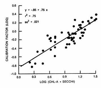
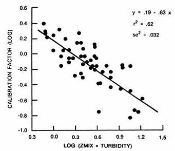
mixed-layer depth in each segment. The relationships depicted in Figure 7
may be used to obtain approximate estimates of reservoir-average calibration
coefficients for use in Model 4 based upon observed monitoring data or
independent estimates of turbidity and mixed-layer depth.
|
|
|
|
Figure 7 - Calibration Factor for Chlorophyll-a Model 4 (Log 10 units) | |
If the reservoir is stratified and oxygen depletion calculations are
desired, temperature profile data taken from the period of depletion
measurements (typically late spring to early summer) are used to estimate the
mean depth of the hypolimnion. If mean hypolimnetic depth is not specified
(= 0.0),the reservoir is assumed to be unstratified and oxygen depletion
calculations are bypassed. The oxygen depletion models are based upon data
from near-dam stations. Accordingly, mean hypolimnetic depths should be
specified only for near-dam segments, based upon the morphometry of the entire
reservoir (not the individual segment). In modeling collections or
networks of reservoirs (Schemes 5 and 6 in Figure 4.3), a mean hypolimnetic
depth can be specified separately for each segment (i.e., each
reservoir).
Calibration Factors
The empirical models implemented in BATHTUB are generalizations about reservoir behavior. When applied to data from a particular reservoir without site-specific calibration, observations may differ from predictions by a factor of two or more. Such differences reflect data limitations (measurement or estimation errors in the average inflow and outflow concentrations), as well as unique features of the particular reservoir. A procedure to calibrate the model to match observed reservoir conditions is provided in BATHTUB. This is accomplished by application of Calibration Factors , which modify reservoir responses predicted by the empirical models, nutrient sedimentation rates, chlorophyll a concentrations, Secchi depths, oxygen depletion rates, and dispersion coefficients . The calibrated model can be applied subsequently to predict changes in reservoir conditions likely to result from specific management scenarios under the assumption that the calibration factors remain constant. Prediction uncertainty ( coefficients of variation predicted by the Error analysis ) will be generaly be over-estimated if the model is calibrated to site-specific data and the default model error CV's are not adjusted downward ( Edit Model Coefficients screen).
For convenience, calibration factors can be applied on two spatial scales: global (applying to all segments) and individual (applying to each segment). The product of the global and individual calibration factors is multiplied by the reservoir response predicted by the empirical model to produce the �calibrated� prediction. All calibration factors have a default value of 1.0. Separate sets of calibration factors can be applied to any or all the following response predictions:
Recognizing that differences between observed and predicted responses are at least partially due to measurement errors, calibration factors should be used very conservatively. The program includes a procedure for deriving least-squares estimates of calibration factors and statistical tests to assist the user in assessing whether calibration is appropriate. Additional guidance is presented in a subsequent section (see Application Steps ).
The first-order error analysis procedure implemented by BATHTUB can be used to estimate the uncertainty in model predictions derived from uncertainty in model inputs and uncertainty inherent in the empirical models. To express uncertainty in inputs, key input variables are specified using two quantities:
Mean = Best Estimate
CV = Relative Standard Error = Standard Error of Mean / Mean
The CV reflects uncertainty in the input value (not the temporal
variability!), expressed as a fraction of the mean or best estimate. CV
values can be specified for most input categories, including atmospheric fluxes
(rainfall, evaporation, nutrient loads), tributary flows and inflow
concentrations, dispersion rates, and observed reservoir quality. FLUX and
PROFILE ( Walker,
1999 ) can be used to estimate Mean and CV values for inflow and reservoir
concentrations, respectively. Model uncertainty is considered by
specifying a CV value for each global calibration
factor ; default CV values derived from CE reservoir data sets are supplied
(see Table 4 and
can be edited by
the user .
Error-analysis calculations provide approximate prediction
uncertainty. Four error
analysis options are available:
0- None (No error analysis)
1- All (Consider input variable & model uncertainty) [default]
2- Model (Consider model uncertainty only)
3- Inputs (Consider input variable uncertainty
only)
CV values specified on input screens are not used in the calculations if error analyses are not requested.
The model model error coefficients reflect the expected uncertainty for application to a reservoir without site-specific calibration and assume that reservoir characteristics (morphometry, hydrology, nutrient levels, etc) are with the ranges of values in the collection of reservoirs used for model development (see supporting research ). As discussed above, if the model is re-calibrated to site-specific data and the default input values for model error coefficients are used, the procedure (Options 2 or 3) will over-estimate prediction uncertainty (CV's of predicted values).